How to Create a Box Plot in Microsoft Excel

Microsoft Excel makes it easy for you to organize, present, and analyze data using various charts. A particularly powerful chart is the box and whisker plot (also known as a box plot), designed to help display the distribution of values in a data set.

In this article, we’ll cover how you can create a box plot in Microsoft Excel, covering both Excel 365 and older versions for those yet to upgrade.

Box Plots: What Are They?

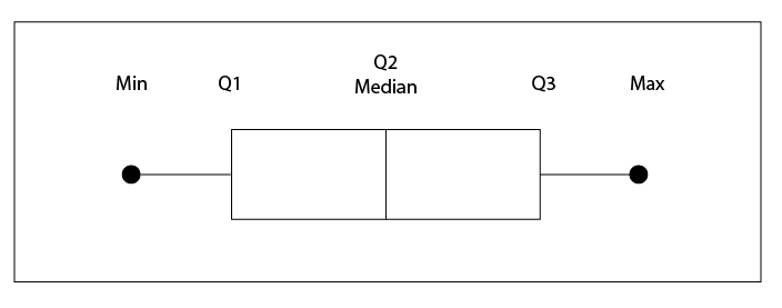
A box plot is a method of displaying data that helps visualize statistical qualities like the spread and variability of the data. It shows a single bar (the box) split in two, with lines (the whiskers) extending to either side of the box.

Each of these elements visualizes the five-number summary of a set of numerical data. They look like this and can be displayed horizontally or vertically:

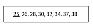
To understand the five-number summary, let’s take a look at a sample data set.

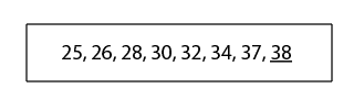
25, 26, 28, 30, 32, 34, 37, 38

1. The minimum. The minimum value in the data set. This is the endpoint to the left/bottom of the left/lower whisker.

2. The first quartile. This is the value under which 25% of data points are found.
3. The second quartile. This is the mediant. It amounts to the “middle value”.
4. The third quartile. This is the value above which 75% of data points are found.
5. The maximum. The maximum value in the data set.

How to Create a Box Plot in Excel 365

In Office 365, Microsoft Excel includes box plots as a chart template, making it easy to create a visual plot for your data. If you aren’t sure how to use Excel, learn the basics first.

To create a box plot:

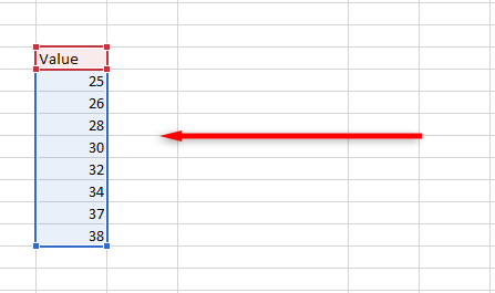
1. Open a new worksheet and input your data.
2. Select your data set by clicking and dragging.

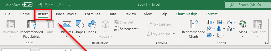
3. In the ribbon, select the Insert tab.

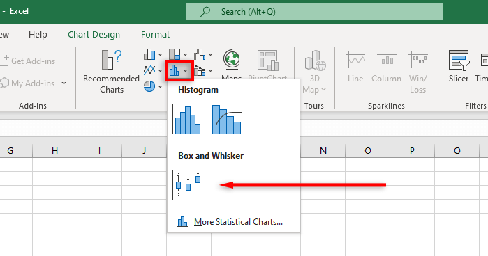
4. Click Insert Statistic Chart then Box and Whisker.

Note: If you insert an empty chart, you can input your data set by selecting the Chart Design tab and clicking Select Data.

Excel will now create a bare-bones box and whisker chart. However, you can customize this Excel chart further to display your statistical data exactly how you’d like it.

How to Format a Box Plot in Excel 365

Excel allows you to style the box plot chart design in many ways, from adding a title to changing the key data points that are displayed.

The Chart Design tab allows you to add chart elements (like chart titles, gridlines, and labels), change the layout or chart type, and change the color of the box and whiskers using built-in chart style templates.

The Format tab allows you to fine-tune your color selections, add text, and add effects to your chart elements.

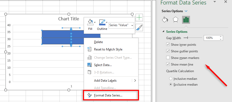
To add further display elements, right-click the box and whisker plot and select Format Data Series from the drop-down menu.

The options include:

1. Show inner points. This displays all individual data points as circles inside the first and third quartiles.
2. Show outlier points. This displays outliers (abnormally high or low data points) as circles outside the plot.
3. Show mean markers. This displays the mean value as a cross within the chart.
4. Show mean line. This displays a line between the average points of multiple data sets.
5. Quartile calculation. If you have an odd number of data points, you can choose to calculate the quartiles by either including or excluding the median. For larger data sets, you should use the exclusive interquartile range, and for smaller data sets the inclusive median method is generally more accurate.

How to Create a Box and Whisker Plot in Older Versions of Excel

As older versions of Excel (including Excel 2013 and Excel 2016) don’t include a template for the box and whisker chart, creating one is much more difficult.

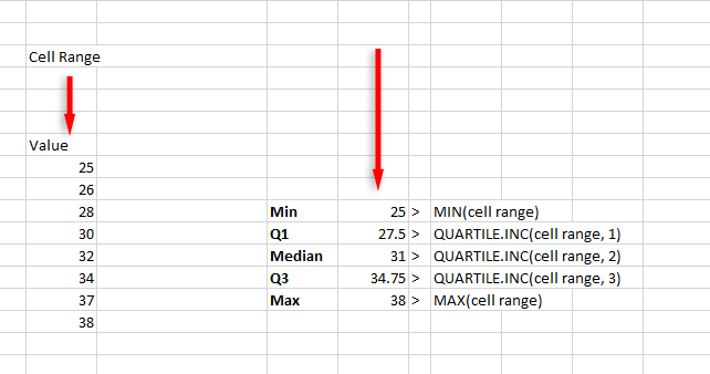
First, calculate your quartile values using the following formulae and create a table:

1. Minimum value: MIN(cell range)
2. First quartile: QUARTILE.INC(cell range,1)
3. Median: QUARTILE.INC(cell range, 2)
4. Third quartile: QUARTILE.INC(cell range, 3)
5. Maximum value: MAX(cell range)

Note: For cell range, drag and select your data set(s).

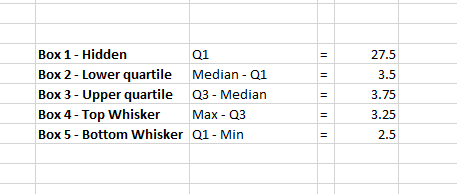
Next, calculate the quartile differences in a separate table (these relate to the box heights):

1. The value of Q1
2. The median minus the Q1
3. Q3 minus the median
4. The maximum value minus the Q3
5. Q1 minus the minimum value

You can then create a chart using these values:

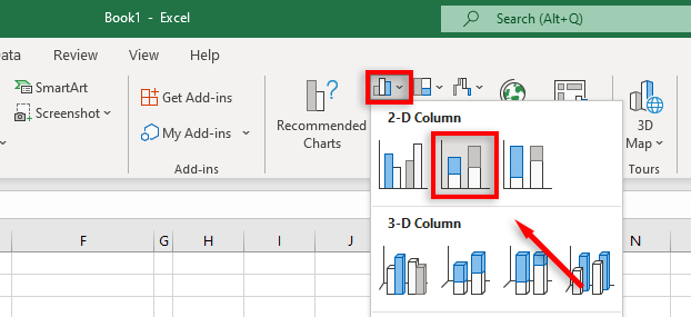
1. Click the Insert tab then select Insert Column or Bar Chart.
2. Click Stacked Column Chart. If the chart isn’t displaying correctly, select the Chart Design tab then click Switch Row/Column.

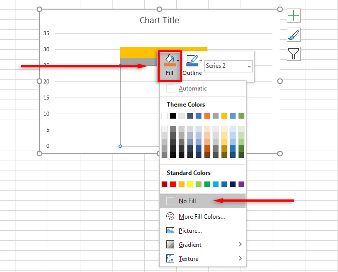
3. Right-click the part of the graph that represents “Box 1 – hidden” and click Fill then click No Fill.

To add the top whisker:

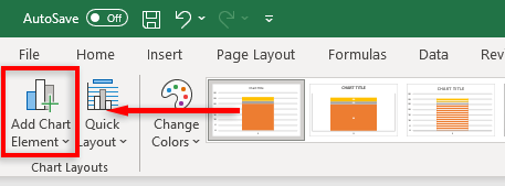
1. Click the top box and select the Chart Design tab.
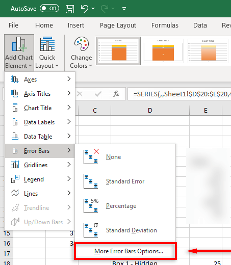
2. Click Add Chart Element.

3. Click Error Bars > More Error Bars Options.

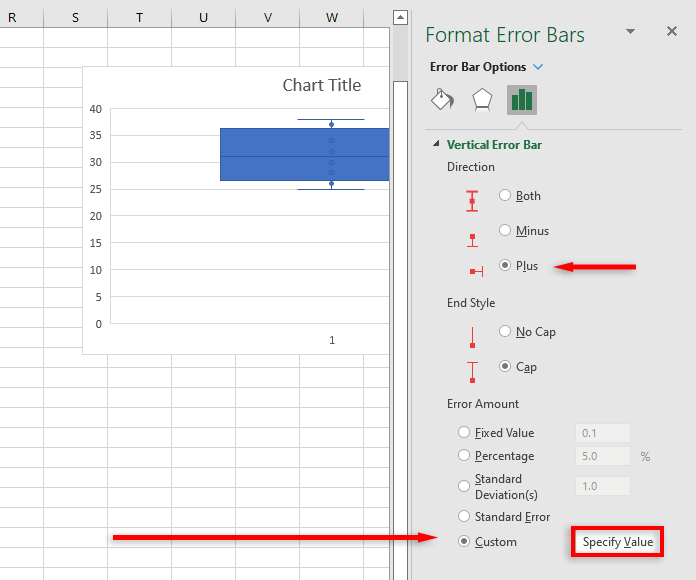
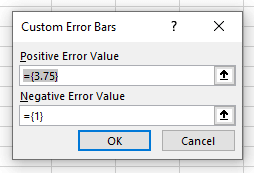
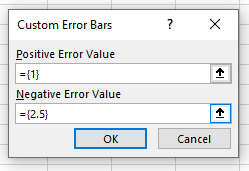
4. Under Direction, click Plus. Under Error Amount click Custom > Specify Value.

5. Replace the Positive Error Value with the value you calculated for Whisker Top.

To add the bottom whisker:

1. Click the hidden box.
2. Under the Chart Design tab, select Add Chart Element.
3. Click Error Bars> More Error Bars Options.
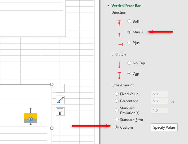
4. Under Direction, click Minus and under Error Amount click Custom > Specify Value.

5. In the dialog box, replace the Negative Error Value with the value you calculated for Whisker Bottom.

You now have a basic box and whisker plot for your data set. You can customize this further by adding a mean line or dot, changing the colors, and altering the chart style.

Statistical Analysis Has Never Been Easier

Luckily, with newer, more powerful versions of the program, visualizing and analyzing data has become much simpler. With this tutorial, you should have a firm grasp of how a box and whisker plot is used and how you can set one up in an Excel workbook.

source https://helpdeskgeek.com/windows-xp-tips/how-to-create-a-box-plot-in-microsoft-excel/